Introduction

In my previous blog post, I discussed the dynamic paired kidney exchange problem, where, over time, an agent must try to maximize the number of compatible pairs selected for kidney donation. In order to test various approaches, I adopted a simulation method based on the work done by Ashlagi et al.. I calculated a theoretical limit of the number of patient-donor pairs that can be matched in any given environment, and compared several common methods to that theoretical maximum. In addition, I evaluated combining two common methods (the periodic batching and greedy methods) and a rudimentary reinforcement learning approach.

Patient Approach

The patient approach, introduced in Unpaired Kidney Exchange: Overcoming Double Coincidence of Wants without Money, proposes a model where, instead of matching a patient right when they join, the patient is matches as they are about to leave.

Following up on my previous blog post, I also tried to combine the patient approach with the greedy approach, using the greedy approach for hard-to-match patients and the patient approach for easy-to-match patients, which didn't yield very good results at all.

Getting Reinforcement Learning to Work

Reading through more papers, I found a great paper from Pimenta et al. on using reinforcement learning with GNNs for this kidney exchange problem. It focuses on a static, not a dynamic graph, but used a similar approach of allowing a GNN to select a subset of nodes before performing a greedy algorithm over that selected subset.

First, I narrowed down the output of the model: rather than having three outputs (which nodes should be selected as "priority" nodes, should the greedy matching algorithm be performed with "priority" nodes, should the greedy matching algorithm be performed with all nodes), the only output for the model was which nodes should be selected for matching with the greedy algorithm.

Second, I changed the way I inputted data to my model: whether or not the node is hard-to-match, how close the node is to its expected departure, and how far through the simulation the environment is. Interestingly, adding information about how far through the simulation the environment is worsened the performance of the model.

Third, I used residual connections in my GNN model. Adding a coefficient and scaling how I added the output of the GNN to a residual model seemed to worsen the performance of my model.

Finally, I normalized the model rewards.

One of the approaches that I tried to improve the performance on the model was to reward the model based on its performance relative to the greedy approach. Intuitively, environments that had a lower performance with the greedy approach would be harder to get a good performance on, even with a model. This led to a minor performance boost, although hyperparameter tuning to see how changing the weighting between the overall reward and the reward relative to the greedy model could be useful. Making the reward relative to the greedy model too large produces too many negative rewards, which seems to hurt the performance of the model.

Looking back at working on trying out different approaches to improve the performance, I wish that I tried to use Git more effectively to create a graph of different experiments, evaluate and annotate the results, and then merge positive changes back into my main branch to work with everything else. Tracking the results of various experiments as I work them out, in this blog post, seems rather unnecessarily haphazard.

Another thing that I noticed impacted model performance heavily was how the model was seeded - a poor seed would lead to a long time with the model having low performance.

With these modifications, the reinforcement learning algorithm is able to independently find the greedy solution - at least for a small node size of 250. In order to accelerate training, I reduced the number of days from 180 days in a year to only 36 days for the entire simulation.

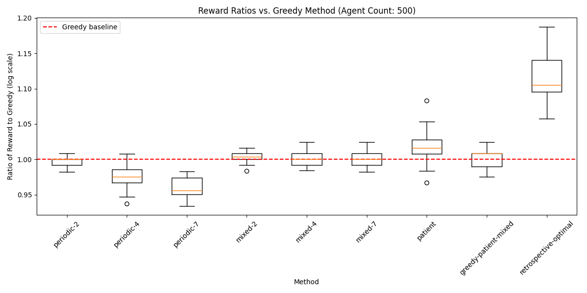
To extend these results to larger simulation environments, I started progressively increasing the number of nodes in the simulation when training the model. In the last evaluation batch, this graph describes the performance gain of the reinforcement learning-based approach over the greedy approach, and over the patient apporach that I discussed above. Interestingly, in this truncated simulation environment, the results of the patient simulation underperform compared to when there are more timesteps.

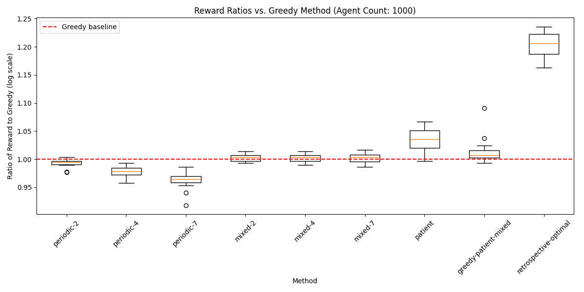
In the final iteration of the model, here is the performance, over 256 simulations, relative to the greedy approach:

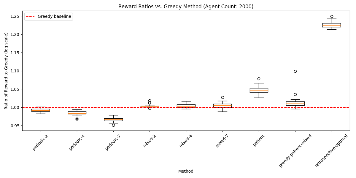
The final configuration for the simulation was with 1000 agents and scaled down for only 36 timesteps. To see if scaling up the number of timesteps would provide more opportunities for the model to improve over the traditional approaches, I scaled up the number of days back up to 180, with a criticality rate of 90 days. That produced the following graph:

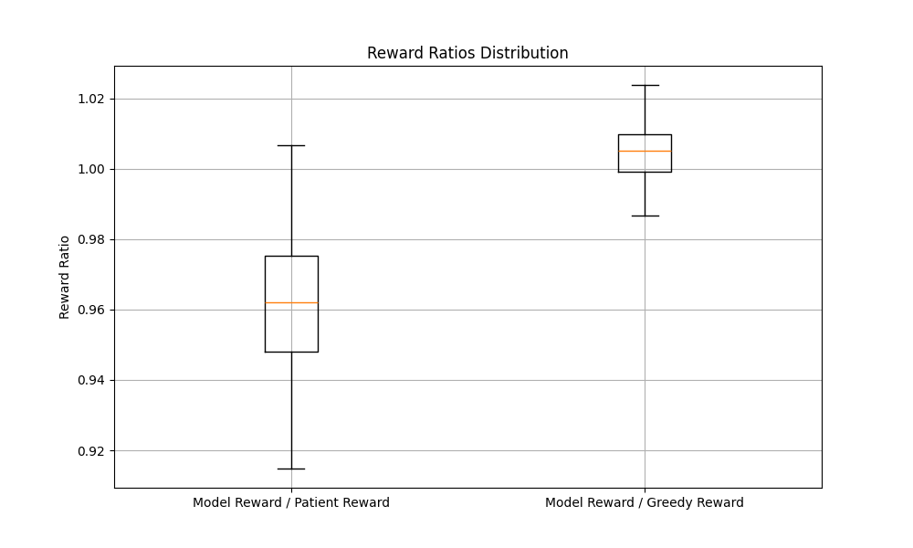
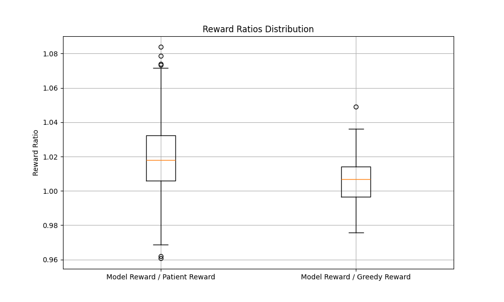
While the reinforcement learning approach is still able to outperform the greedy approach, it is unable to outperform the patient apporach, even though it has the data required to be able to outperform the patient approach (namely, when the patient will leave the system).